Introduction
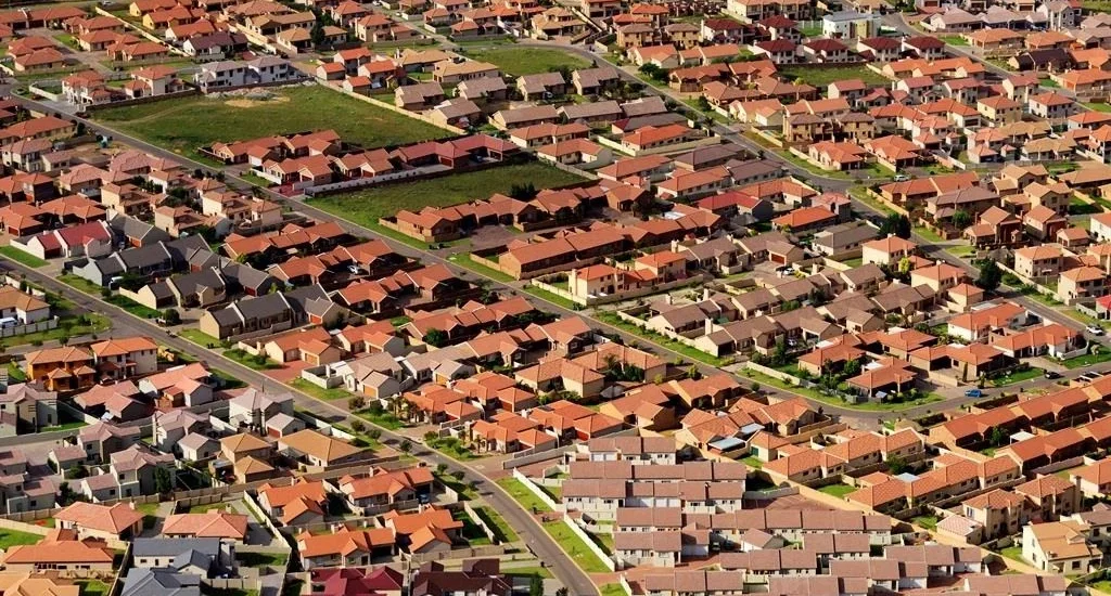
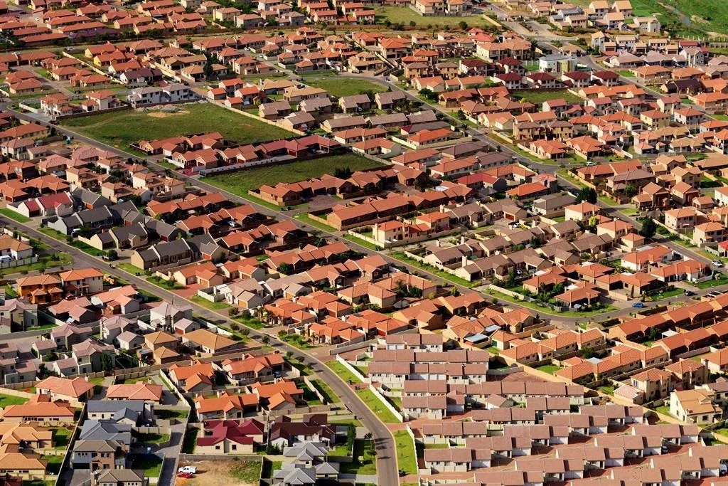
The city in the middle of the desert is growing fast, but urban sprawl has not appeared there yet. From open desert in 1972 until late 2000, the city moved forward very fast in terms of urban growth. The government opened the doors for people from all over the world to come and live in the city and eased the residence requirements. Developers opened their eyes to this growing city and the opportunity it created for making money. After the massive growth, local residents felt the city dynamics, and the environment it created was no longer peaceful for them. Developers also wanted the idea of a fantasy calm, quiet place to live, away from city movement, pollution and problems. Yes, now we witness urban sprawl moving through the city like a snake. But this movement is not seen as a damaging phenomenon in the way the western world sees it.
Urban sprawl has circled in the western world, even in academic research, for a long time. Various concepts emerged to support the birth of this idea. From Wright’s Broadacre City to the Garden City, they all wanted to move out of the city to the countryside. They wanted a peaceful mind, calm areas, beautiful views of the countryside and, definitely, car-oriented development. Here urban sprawl came into view. Urban sprawl is closely linked to changes in urban density in the city. The gentrification approach of shifting people also has a direct connection to urban sprawl. I have presented urban density in detail in my article Urban Density in Practice.
When was the term “urban sprawl” coined?
According to academic literature, the term was first coined in 1937. “Urban sprawl” is commonly credited to Earle Shenton Draper Jr., a U.S. town planner who used it in 1937. It was popularized and given definitional weight in the mid-20th century, as American suburbs expanded after World War II.
The research does establish a contested history:
The term’s pejorative use became common in American public debate only in the post-war era. Anti-sprawl commentary in this vein intensified from the 1950s onward, as part of a long antisuburban and antiautomobile tradition. An early published use appears in a 1953 piece titled simply “The Urban Sprawl” (“The Urban Sprawl,” 1953), less than two decades after the supposed 1937 coinage.
The most direct historical treatment argues the opposite reading. Bruegmann’s account contends that sprawl, far from being recent or distinctly American, is “as old as cities themselves.” It is characteristic of ancient Rome and 18th-century Paris as much as of Atlanta or Los Angeles. The term’s pejorative connotations, he argues, are a modern overlay on a pattern as old as urbanization (“Sprawl: A Compact History,” 2006).
Academic and policy attention to sprawl as a problem intensified sharply in the 1980s and 1990s, when it became a recognized planning agenda item. Even so, reviewers note that the field never agreed on a definition (Dadashpoor & Shahhossein, 2024; Chettry, 2023).
Research on urban sprawl has remained large regardless of technology development and the massive number of research papers published. The counts have fallen since 2022. In Google Scholar they dropped from 22,800 papers in 2022 to 18,000 in 2025, and in OpenAlex from 4,350 to 3,260 over the same years. The 2026 figures (13,300 and 2,410) cover only part of the year, so they are not comparable with full years. Even so, thousands of papers a year still indicate its importance in the academic context and in professional practice. Many non-professionals think that the amount of research reflects the concept’s vague meaning and misinterpretation in the field it relates to. Following are figures from two sources indicating the number of research papers published from 2022 to 2026.
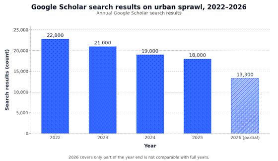
Figure 1. Annual Google Scholar search results on urban sprawl, 2022–2026 (2026 is a partial year).
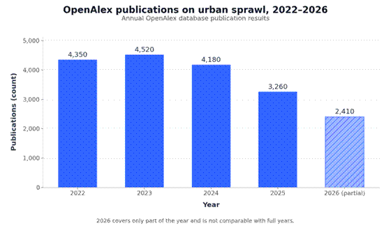
Figure 2. Annual OpenAlex database publication results on urban sprawl, 2022–2026 (2026 is a partial year).
Looking at the full output across all journals globally in OpenAlex, the papers published from 2022 to 2026 divide into three distinct method blocks:
- Spatial modeling (~40% of papers): driven heavily by GIS and CA-Markov simulations forecasting how highway proximity and zoning policies will artificially force cities outward through 2050.
- Environmental optimization (~35% of papers): investigating immediate micro-climate degradation, carbon emission dependencies, and the loss of peripheral agricultural green infrastructure.
- Socio-economic and policy interventions (~25% of papers): exploring spatial segregation, infrastructure cost overruns, and the viability of transit-oriented development (TOD).
Urban sprawl definition
Anyone looking for a definition, whether a researcher or a professional in the field of urban planning, will find an overwhelming number of them. In research and academic papers there are more than 130 definitions, each focusing on a specific dimension of urban sprawl. Most definitions share a common core of physical form. Sprawl is repeatedly characterized by three interlocking spatial attributes: low density, low continuity of the built-up area (scattered, leapfrog development), and low compactness of urban shape. On this basis, one influential operational definition holds that sprawl is higher when more area is built over in a landscape. It is also higher when the built-up area is more dispersed, and when land uptake per inhabitant or job is higher (lower utilization intensity). An alternative framework identifies five dynamic attributes commonly labeled sprawl (Angel et al., 2007). They are the extension of cities beyond walkable range, persistent decline in density, ongoing suburbanization away from metropolitan centers, fragmentation of open space, and infill that fills in between fingerlike extensions.
Definitions vary by discipline, each focusing on one aspect. A systematic review of 130 definitions set out to resolve this by classifying them into a sixfold scheme: pattern-oriented, process-oriented, nature-oriented, location-oriented, actors-oriented, and factors-oriented (Dadashpoor & Shahhossein, 2024). Related work stresses that a defensible definition must disentangle the phenomenon itself from its causes and consequences, since both differ across regions and regulatory contexts. Table 1 summarizes the definitional dimensions.
Table 1. Definitional dimensions of urban sprawl
| Definitional dimension | What it captures | Example treatment |
| Pattern / form | Density, continuity, compactness | Three-attribute characterization (Steurer & Bayr, 2020) |
| Process | How growth occurs (scattered, leapfrog, infill) | Five dynamic attributes (Angel et al., 2007) |
| Cause vs consequence | Separating sprawl from its drivers and impacts | Clarification of definition (Jaeger et al., 2009) |
| Normative judgment | Sprawl as “everything bad about urban growth” | Decomposition of sprawl into component parts (Peiser, 2001) |
From definition to measurement
Because the definition is contested, much of the literature pivots to measuring the phenomenon, and this is where the concept becomes operational. A key theme is that sprawl is multidimensional and best quantified by multiple measures rather than one index. Methodological work grounds measurement in a clear definition. Thirteen suitability criteria were derived for evaluating sprawl metrics. A companion paper used them to build the weighted measures DIS (degree of urban dispersion), TS (total sprawl), UP (urban permeation of the landscape), and SPC (sprawl per capita) (Jaeger et al., 2009). This program matured into the Weighted Urban Proliferation (WUP) metric. It integrates the three dimensions of built-up amount, spatial dispersion, and utilization intensity into one measure, and it documented a 155% increase in Swiss sprawl between 1935 and 2002.
Urban planners use quantitative, spatial, and remote-sensing tools to measure and monitor the degree of sprawl over time:
- Remote sensing and GIS: satellite imagery, aerial photography, and topographic maps track changes in built-up footprints across temporal scales.
- Image processing techniques: standard workflows include image extraction, rectification, restoration, and classification.
- Shannon’s entropy: a statistical measure used to quantify the degree of spatial concentration or dispersion of urban land use.
- Weighted Urban Proliferation (WUP): an index measuring built-up area intensity, land per capita, and the spatial configuration of dispersion.
- Spatial indicators: analysis of built-up area ratios, shape indexes, and accessibility metrics rather than relying on arbitrary boundary definitions.
The European Environment Agency applied WUP to 32 European countries (the EU-28 plus Iceland, Liechtenstein, Norway and Switzerland) for 2006 and 2009. WUP is measured in urban permeation units per square metre of landscape (UPU/m²), and a higher value means more sprawl. Table 2 compares the 15 EU countries with the highest WUP values in 2009. All of them are above the value for the 32 countries combined (1.64 UPU/m² in 2009). The Netherlands and Belgium come first by a clear margin, followed by Malta, which also recorded the largest increase between 2006 and 2009.
Table 2. Urban sprawl in the 15 most sprawled EU countries, 2009 (EEA country-level values)
| Rank (2009) | Country | WUP 2006 (UPU/m²) | WUP 2009 (UPU/m²) | Built-up area 2009 (%) | Land uptake per inhabitant or job 2009 (m²) |
| 1 | Netherlands | 6.40 | 6.61 | 14.82 | 227.6 |
| 2 | Belgium | 6.48 | 6.59 | 13.23 | 276.3 |
| 3 | Malta | 4.14 | 5.58 | 24.27 | 135.7 |
| 4 | Luxembourg | 3.86 | 4.01 | 9.39 | 302.5 |
| 5 | Germany | 3.74 | 3.83 | 9.14 | 284.4 |
| 6 | United Kingdom | 3.07 | 3.18 | 7.45 | 209.5 |
| 7 | Denmark | 2.98 | 3.04 | 6.76 | 365.7 |
| 8 | Cyprus | 2.49 | 2.74 | 5.88 | 457.8 |
| 9= | France | 2.26 | 2.33 | 5.23 | 328.1 |
| 9= | Portugal | 2.20 | 2.33 | 4.98 | 298.6 |
| 11 | Italy | 2.04 | 2.18 | 5.66 | 208.4 |
| 12 | Hungary | 2.02 | 2.12 | 5.59 | 380.4 |
| 13 | Czech Republic | 2.05 | 2.11 | 5.71 | 294.2 |
| 14 | Croatia | 1.81 | 1.92 | 4.46 | 423.7 |
| 15 | Ireland | 1.78 | 1.89 | 3.68 | 419.6 |
Source: European Environment Agency and Swiss Federal Office for the Environment (2016), Urban sprawl in Europe, EEA Report No 11/2016, Annex 1, Table A1.1. Reproduced with acknowledgment of the source. WUP is weighted urban proliferation; a higher value means more sprawl. Countries are ranked by WUP 2009, and France and Portugal share 9th place (2.33). The United Kingdom was an EU member during the 2006–2009 study period. Liechtenstein (6.06) and Switzerland (2.57) are EFTA, not EU, countries and are left out.
Country values hide large regional differences. A country with high sprawl in a few regions can still have a low national value. Small countries such as Malta tend to show more extreme values than large ones. The figures in Table 2 are therefore best read as a first comparison, not a final ranking. The report itself stresses the regional (NUTS-2) and 1 km² results for a closer look.
Urban sprawl relation with urban design
The relation of urban sprawl to urban design is twofold. Conventional suburban design produces sprawl, and anti-sprawl design movements (compact city, New Urbanism, smart growth) are the principal design response to it. Yet the empirical evidence shows that design alone is a weak, context-dependent cure that frequently fails to deliver its promised density and containment.
How sprawl and design are coupled. Sprawl is fundamentally a product of how the built environment is laid out, so urban design sits at both ends of the problem. The critique of sprawl assumes an ideal urban form, the compact, self-sufficient city, against which sprawling form is judged. Design movements position themselves explicitly as the corrective. The compact city is a leading paradigm of sustainable urbanism. Its core design strategies are compactness, density, diversity, mixed land use, sustainable transport, and green structure. New Urbanism advocates a return to human-scale, pedestrian-friendly, small-town urban form “and a stop to suburban sprawl” (“New Urbanism and beyond: Designing Cities for the Future,” 2009). In Europe and North America, the policy responses to sprawl are themselves design doctrines. These are New Urbanism and smart growth in North America, and compact city and multifunctional land use in Europe.
How far design actually counters sprawl: the empirical track record. The evidence on whether these design strategies deliver is mixed, and several rigorous studies are skeptical. The relationship is best shown as a table because the case studies share the same dimensions (strategy tested, claim, empirical result).
Table 3. Design strategies against sprawl: intended effect and empirical outcome
| Design strategy | Intended effect | Empirical outcome |
| Compact city, Gothenburg/Helsingborg | Compactness and mixed use support all three sustainability goals | Achieved, but economic goals dominate environmental and social ones in practice (Bibri et al., 2020) |
| Compact city, Jeddah | Raise density and reduce sprawl | Density rose from 44 to 155 people/ha, but the city still grew 20% with land prices up 300%; failed to control sprawl as anticipated (Shawly, 2022) |
| Spatial strategies, Istanbul | Restrict sprawl via development control | Up to 62% sprawl reduction, but only with strong spatial restrictions and added requirements, not the current planning approach (Terzi & Bölen, 2011) |
| New Urbanism, Cornell (Canada) | New urbanist design raises density and substitutes for conventional suburbia | Raises suburban densities, but far less than simple comparisons suggest; only 37% single-family detached homes, and most households there plan to move to detached houses (Skaburskis, 2006) |
Two further results sharpen the lesson. Compactness is a necessary but insufficient condition, because physical urban compactness alone cannot meet containment aims when residents’ relocation freedom and sociocultural preferences are ignored. And across many cities planning has only weak impact. In Japan, sprawl and scatteration persist “despite a planning system that is formally supposed to prevent it.” This points to institutional and land-market factors that design cannot override. Even the flagship anti-sprawl toolkit is contested. Yet the broad critical attack on New Urbanism has been characterized as largely unconvincing and resting on caricature rather than adequate sampling (Ellis, 2002).
The design toolkit beyond density. Design counters sprawl not only by densifying but by reshaping what already sprawls. Sprawl retrofit treats existing suburban fabric as the site of intervention. It evaluates locations by overlaying accessibility, density, diversity, and connectivity. It then applies neighborhood and site-scale design, code reform, intensification around transit nodes, public investment in civic space, and traffic calming. Redeveloping industrial and former military sites and retrofitting structures for mixed use are promoted alongside promoting sustainable urban growth (Wetzel, 2024).
Design’s relation is contested, not settled. The relation is genuinely debated rather than resolved. Because sprawl itself lacks an agreed definition, the design response is hard to evaluate consistently. The debate over whether compact versus sprawling form drives sustainable outcomes has dominated planning literature for roughly a decade and a half. Compact-city critiques around feasibility and acceptability apply readily to intensification efforts whose higher densities clash with residents’ perceived ideal lifestyle (Hampton, 2010). The single most consistent conclusion is that design is a real but bounded lever. It can reduce sprawl only when paired with regulatory restriction, market realism, and attention to how people actually choose to locate.
Urban sprawl relation with urban planning
The relation between urban sprawl and urban planning is one of mutual constitution. Sprawl has long been framed as a planning problem and the spur for a generation of containment doctrines (compact city, New Urbanism, smart growth). Yet the empirical record shows planning remedies are uncertain, context-dependent, and sometimes ineffective. This is because sprawl is driven as much by land markets and institutional factors as by physical layout.
How planning frames sprawl as its core problem. Across the literature, sprawl sits at the center of the planning research agenda and its sustainable-development critique. It has been “on the planning research agenda for more than five decades.” Because planners largely reject sprawl as a desirable urban form, the definitional debate itself is an outgrowth of planning’s normative stance toward it. The dominant planning response is the “predict and contain” family of paradigms:
Table 4. Planning doctrines and their stated relation to sprawl
| Planning doctrine | Stated relation to sprawl |
| Compact city | The leading paradigm of sustainable urbanism, promoted as the preferred response to sprawl and unsustainability (Bibri et al., 2020) |
| New Urbanism | Advocates small-town, human-scale, pedestrian form “and a stop to suburban sprawl” (“New Urbanism and beyond: Designing Cities for the Future,” 2009) |
| Smart growth (North America) | Regulatory family aimed at containing deconcentration (Dieleman & Wegener, 2004) |
| Multifunctional land use (Europe) | European counterpart to smart growth against sprawl (Dieleman & Wegener, 2004) |
| Urban edges / growth boundaries | A planning-management structure shown to leave cities “better off” than those without containment policy (van Rensburg & Campbell, 2011) |
The compact city and smart growth approaches have been widely implemented over the last three decades as the preferred instruments against sprawl.
But the empirical track record is skeptical. Detailed case studies find that containment models frequently do not achieve their aims. A study of Jeddah evaluated the compact city model’s implementation to control sprawl. It found the effort did not succeed, concluding that planning there has not effectively managed undesired growth. An analysis of the Cornell new urbanist development found it increased suburban densities “but not by nearly as much” as a naive comparison implies. Many residents still planned to move to detached houses, so new urbanism’s effect on sprawl is far smaller than proponents claim. Scenario testing of compact spatial strategies in Istanbul showed their ability to control sprawl depends critically on commercial profitability, which the compact approach must address. Japan’s case is the starkest. A review found the planning system, legally committed to prevention, nonetheless produced “the actual ineffectiveness of planning.” This was explained by institutional and land-market factors rather than design defaults.
Why planning remedies so often fail: the causal decomposition. The explanation that recurs is that sprawl is not purely a spatial-design phenomenon, so planners who treat it as one misdiagnose it. Sprawl is partly a response to market and institutional forces: housing-consumption preferences (freedom to locate anywhere), the private car, and land markets all generate deconcentration. Planners must distinguish the aspects of sprawl that are genuinely deleterious from those that are not, a decomposition that determines which containment goals deserve policy weight. Spatial planning is the planning activity that integrates land use with transport, housing, and the environment. Framing sprawl in this way, rather than merely as a land-regulation problem, is offered as the route to a more effective response. This is why one review concludes that planners and politicians “must agree upon a definition and a method for measuring progress” if containment is to be tractable at all (Siedentop, 2005).
Methods and tools planners use
Planners rely on four statistical methods to track urban growth, project future demand and judge the economic effects of development. Each has a different job and a known weakness. The table summarizes them, and the sections that follow explain how they work in practice.
Table 5. The four methods at a glance
| Method | Main planning uses | Typical techniques | Main weakness |
| 1. Time series analysis | Tracking urban expansion from satellite images; separating trends, seasons and shocks in traffic and energy data | Landscape metrics on image series, seasonal decomposition, ARIMA | Needs long, consistent records |
| 2. Forecasting and futures research | Projecting demand for energy, transport and land | ARIMA and exponential smoothing; newer machine-learning models | Newer models are often tested on only one or a few cities |
| 3. Economic impact assessment | Comparing costs and benefits of plans; land values; effects on jobs and business | Cost-benefit analysis, multi-criteria frameworks, before-and-after studies | Gains in one area are often activity displaced from another |
| 4. Trend extrapolation | Projecting population, land use and built-up area | Linear regression, ARIMA, trend surfaces | Assumes the past continues; unreliable over long horizons or after a policy change |
1. Time series analysis
A time series is a measurement repeated over time, such as population, traffic counts or the area covered by buildings. Analyzing it separates the long-term trend from seasonal patterns and one-off shocks, which shows a planner what is a lasting change and what is noise.
For sprawl, the most useful application is satellite imagery. A sequence of classified images shows how fast a city’s built-up area is growing and what shape that growth takes. A study of four fast-growing cities in southern China used ten Landsat images from 1988 to 1999. It found that combining growth rates with landscape metrics described urban expansion better than growth rates alone. It also found that the cities converged toward a similar urban form. Because urban change is often nonlinear, with several transitions, newer change-detection methods look for the timing of each shift instead of assuming a smooth trend. Planners apply the same logic to traffic counts and electricity demand.
Traffic and mobility forecasting is where the shift from classical models to deep learning is clearest.
Table 6. Traffic and mobility forecasting: classical and deep-learning approaches
| Application | Classical approach | Deep-learning turn |
| Traffic flow/volume | ARMA models (Zhi-yong, 2004); pattern-based prediction (Thomas et al., 2009) | GCN with adversarial training (Yu et al., 2020) |
| Regional traffic flow | — | STGCN-BiLSTM hybrid (Wu, 2021) |
| Passenger mobility | — | Context-aware origin-destination forecasting (Wang et al., 2022) |
| Travel time | Time series models vs simulation (Hu & Ho, 2010) | Deep learning synthesis (Liu et al., 2018) |
2. Forecasting and futures research
Forecasting turns time series into projections of future demand. In urban planning it is concentrated in three sectors: energy demand, transport and traffic, and urban expansion. Classical models such as ARIMA, exponential smoothing and seasonal decomposition remain the standard benchmark, particularly for annual and strategic planning. Newer data-driven methods, such as deep learning that adds spatial structure to the time dimension, often do better on short-term, high-frequency forecasts like road speeds or hourly electricity demand. Studies report these gains mostly for one or a few cities, so they have not been widely replicated.
In practice, planners use classical methods for long horizons, newer models for day-to-day operations, and satellite monitoring to check the physical footprint that other forecasts assume stays fixed.
For energy demand, one of the three sectors, the main model families and their uses are listed below.
Table 7. Energy demand forecasting: model families and uses
| Model family | Energy use cases | Reference |
| ARIMA / seasonal time series | Year-ahead gas demand, daily electricity | (Akpınar & Yumuşak, 2016; Nooruldeen et al., 2022) |
| Data-driven (linear, ML) | City daily electricity with weather extremes | (Wang et al., 2021) |
| Decomposition + LSTM | Energy load benchmarking | (Bhat et al., 2024) |
| Graph convolutional network | Inter-building urban energy | (Hu et al., 2021) |
| Planning-support systems | E-GIS mesh forecasting; distributed supply siting | (Takahashi et al., 2019; Yeo et al., 2013) |
3. Economic impact assessment
Economic impact assessment asks what a plan or project is worth and who gains. The classic tool is cost-benefit analysis, which Nathaniel Lichfield adapted for city planning in 1960 so that alternative plans could be compared on their benefits and costs. Newer versions add stakeholders and non-monetary criteria, because a single benefit-cost ratio hides who wins and who loses.
The main newer frameworks are summarized here.
Table 8. Newer evaluation frameworks
| Framework | Contribution |
| Multi-stakeholder CBA (urban development projects) | Combines CBA with stakeholder interest mapping via focus groups and AHP; estimates cost/benefit distributions per stakeholder plus net present value and benefit-cost ratio for eight Indonesian residential developments (Pramono et al., 2022) |
| Multicriteria economic assessment (historic urban landscape) | Six indicator categories for culture-led regeneration, framed around multidimensional benefits beyond monetary output (Girard et al., 2016) |
| Valuing urban regeneration benefits | Method to build on routine UK evaluation evidence and statistics, with explicit caveat that benefit-cost ratios are subject to substantial conceptual and measurement problems (Tyler et al., 2012) |
| Financial feasibility / break-even model | Ex-ante financial viability test for regeneration projects that relaxes the linearity assumptions of classic break-even analysis for public-private decisions (Tajani et al., 2023) |
| Ex-ante socioeconomic impact modeling | Financial valuation of socio-economic impacts (jobs, population, visitor increments) to compare against initial investment for large projects (Pelčák & Korytářová, 2021) |
Research is most developed in three areas. These are how planning decisions affect land and property values, how planning restrictions and enterprise zones affect business and jobs, and what regeneration programs achieve. The evidence is skeptical. Many studies find modest effects, and what looks like growth is often activity moved from elsewhere. In France, for example, an enterprise-zone program succeeded in attracting firms into the zones, but the effect came entirely from firms relocating within the same municipalities.
The lesson for planners is to separate gross benefits from net benefits, and the value a project creates from the value it merely shifts.
4. Trend extrapolation
Trend extrapolation is the simplest forecasting method: it extends a historical trend, usually with linear regression or a time series model, into the future. Planners use it to estimate future population, vehicle ownership and the land needed for development. It is cheap, transparent and easy to explain, and it works well when conditions are stable and the horizon is short.
Typical applications are shown below.
Table 9. Applications of trend extrapolation
| Application | Method | Setting / finding |
| Urban land-use change | Regression vs. Markov chains | Linear regression more robust than Markov for projecting urban growth tendency (López et al., 2001) |
| Urban population growth | ARIMA (20,1,10) | Philippines, RMSE 0.19, MAPE 3.71%, rising trend to 2.36% by 2028 (Estoque et al., 2022) |
| Vehicle ownership | Sub-extrapolation per traffic zone | Transport & travel-demand planning (Hua-bing, 2010) |
| Bus-transit demand | Time series extrapolation | Zagreb; short-term only, assumes stable drivers (Milojević & Pavlica, 1983) |
| Sustainable-development indexes | Grey GM(1,1) + fuzzy-element forewarning | Trend projection with a forewarning alert layer (Xu, 2008) |
| Urban expansion pattern | Trend-surface mapping | Western Kobe, cubic-to-quartic surfaces over time and space (Tanaka, 1979) |
Its weakness is the assumption that the past continues. An extrapolation cannot see a new transport line, a change in policy or an economic shock, and its errors grow as the horizon lengthens. Researchers have also long warned that forecasts reflect the assumptions fed into them and the decisions they are meant to support. The scale of the problem is clear from transport projects. A study of 210 projects in 14 countries found rail passenger forecasts overestimated in nine of ten cases, by 106% on average. For this reason, planners increasingly treat an extrapolation as one input among several scenarios, not as the forecast itself.
How the methods fit together for sprawl
Applied to sprawl, the methods work as a chain. Satellite time series measure how quickly built-up land is growing, and the European Environment Agency’s sprawl figures rely on this kind of satellite data. Forecasting and extrapolation give an estimate of where that growth leads. The caution is that the EEA’s own comparison covers only three years (2006 to 2009) and may not represent longer trends. Impact assessment then asks what the growth costs and who pays.
Urban sprawl: the innovative solution
Since 2006, in professional practice, the urban sprawl phenomenon has attracted my attention. Professionals debate its negative consequences for the economy, as it increases government spending on infrastructure for low-density development. They debate its effect on the environment, because the increase in roads and highway surfaces produces a heat island effect and car pollution in the atmosphere. It is a cause of social segregation that weakens society and the ties between people. It also increases the use and development of virgin land, which damages biodiversity and the growth of natural elements.
The Business Hubs: an innovative solution. Working in professional practice, getting involved in mega urban development, and doing academic research drove my desire to find a resolution. Since the periphery of a city is well served by public transport and infrastructure, this will prevent public spending when targeting development. A business hub urban development would be located on these boundaries, provided it fulfills conditions such as the location being a deprived area. Spotting deprived areas on the boundary of cities will enhance their economic competence.
Another condition is the availability of low-density housing in the nearby area, which will prevent new housing development and direct effort towards renovating existing stock. In this manner the price of rentable areas will increase gradually, and employment in the area will bring additional income. There will be no car reliance, no negative effect from building roads, and no pollution coming from them. There will be a gradual increase in the desire to develop the area and a steady improvement of infrastructure and mass transit.
People will start to shift gradually from the centers to the boundaries in reasonable numbers, which reduces the effect of gentrification. An increase in social mix will improve well-being and the sense of equity. There is no load on public funds for the transport network. People’s mortgages fund home purchase, and social benefits decrease as people find jobs. Most importantly, the load on public funds for developing areas is reduced, allowing the focus to stay on priorities in the city center.
This is an innovative solution that does not need public consent, or massive research efforts and funding. It is a matter of contributing to professional practice and providing well-being for human beings, regardless of race, gender, country, and religion.
Further reading
- Seto, K. C. & Fragkias, M. (2005). Quantifying spatiotemporal patterns of urban land-use change in four cities of China with time series landscape metrics. Landscape Ecology, November 2005. doi:10.1007/s10980-005-5238-8. Satellite time series applied to urban growth.
- Flyvbjerg, B., Holm, M. K. S. & Buhl, S. L. (2005). How (in)accurate are demand forecasts in public works projects? The case of transportation. Journal of the American Planning Association, 71(2). The best-known evidence on how wrong forecasts can be.
- Wachs, M. (1987). Forecasts in urban transportation planning: uses, methods, and dilemmas. Climatic Change, 11(1–2). How forecasts are used, and shaped, in planning practice.
- Lichfield, N. (1960). Cost-benefit analysis in city planning. Journal of the American Institute of Planners, vol. 26, p. 273. The origin of cost-benefit analysis for planning.
- Mayer, T., Mayneris, F. & Py, L. (2017). The impact of Urban Enterprise Zones on establishment location decisions and labor market outcomes: evidence from France. Journal of Economic Geography, 17(4), 709–752. Why enterprise-zone gains can be displacement.